Topic #1 Module: Computing a Julia Set

Overview

Objective: To implement several versions of a "toy" parallel application that computes the Julia set displayed below and saves it as a bitmap file:

What is a Julia set?

A Julia set is a fractal, i.e., an object that is self-similar across scales (you "zoom in" and you keep seeing similar structures/features). It is a generalization of the famous Mandelbrot set[Wikipedia], which adorns many T-shirts (search for "Mandelbrot zoom" for psychedelic videos).

The particular Julia set that we compute here is defined as follows. Given z a point in the 2-D complex plane, we compute the series defined as:

  • z0 = z
  • zn+1 = zn2 + c
where c = -0.79 + i * 0.15. Different values of c lead to different images, and we know many values that produce "pretty" images.

The color of a pixel corresponding to point z is determined based on the number of iterations before the modulus of zn is above 2 (or until a maximum number of iterations is reached).

Not to worry, code is provided for you for the above. However, feel free to tweak it to create different images and to find out more about Julia sets[Wikipedia].

Roadmap

This module consists of 3 activities, each described in its own tab above, which should be done in sequence:

  • Activity #1: Realize a sequential implementation of a program that computes the Julia set and outputs it to a bmp file.
  • Activity #2: Realize a parallel implementation the program with MPI, using a 1-D data distribution.
  • Activity #3: Realize a parallel implementation the program with MPI, using a 2-D data distribution.

What to turn in

You should turn in a single archive (or a github repo) with:

All source code
XML platform files and host files (see details in the activities)
A Makefile that compiles all executables (and has a 'clean' target!)
A README file with answers to the questions asked in the activities

In this activity we develop a simple sequential (i.e., non-parallel) program that computes a Julia set and saves it to a bitmap file. We break it down into the two steps below:
Implement a C (or C++) program called sequential_julia (source file sequential_julia.c) that:
Takes a single command-line argument, n, an integer that's strictly positive.
Allocates an 1-D unsigned char array of n*(2*n)*3 elements. This array is used to store the pixels of an image with height (in pixels) of n width (in pixels) of 2n, where each pixel is encoded using 3 bytes (RGB values).
Fills this array with pixel values corresponding to the Julia set.

To make the above easier you are provided with one helper C function, compute_julia_pixel(), to which you pass the (x,y) coordinates of a pixed, the (width, height) dimensions of the image, a "tint" float (pass 1.0 for now), and a pointer to 3 contiguous bytes (unsigned char *). These bytes are set to appropriate RGB values (Red Green Blue) for displaying the Julia set. [Download source of compute_julia_pixel()]

See the source of compute_julia_pixel()...
/*
 * compute_julia_pixel(): compute RBG values of a pixel in a
 *                        particular Julia set image.
 *
 *  In:
 *      (x,y):            pixel coordinates
 *      (width, height):  image dimensions
 *      tint_bias:        a float to "tweak" the tint (1.0 is "no tint")
 *  Out:
 *      rgb: an already-allocated 3-byte array into which R, G, and B
 *           values are written.
 *
 *  Return:
 *      0 in success, -1 on failure
 *
 */

int compute_julia_pixel(int x, int y, int width, int height, float tint_bias, unsigned char *rgb) {

  // Check coordinates
  if ((x < 0) || (x >= width) || (y < 0) || (y >= height)) {
    fprintf(stderr,"Invalid (%d,%d) pixel coordinates in a %d x %d image\n", x, y, width, height);
    return -1;
  }

  // "Zoom in" to a pleasing view of the Julia set
  float X_MIN = -1.6, X_MAX = 1.6, Y_MIN = -0.9, Y_MAX = +0.9;
  float float_y = (Y_MAX - Y_MIN) * (float)y / height + Y_MIN ;
  float float_x = (X_MAX - X_MIN) * (float)x / width  + X_MIN ;

  // Point that defines the Julia set
  float julia_real = -.79;
  float julia_img = .15;

  // Maximum number of iteration
  int max_iter = 300;

  // Compute the complex series convergence
  float real=float_y, img=float_x;
  int num_iter = max_iter;
  while (( img * img + real * real < 2 * 2 ) && ( num_iter > 0 )) {
    float xtemp = img * img - real * real + julia_real;
    real = 2 * img * real + julia_img;
    img = xtemp;
    num_iter--;
  }

  // Paint pixel based on how many iterations were used, using some funky colors
  float color_bias = (float) num_iter / max_iter;
  rgb[0] = (num_iter == 0 ? 200 : - 500.0 * pow(tint_bias, 1.2) *  pow(color_bias, 1.6));
  rgb[1] = (num_iter == 0 ? 100 : -255.0 *  pow(color_bias, 0.3));
  rgb[2] = (num_iter == 0 ? 100 : 255 - 255.0 * pow(tint_bias, 1.2) * pow(color_bias, 3.0));

  return 0;
}

The program must store the pixels of the 2-D image into the 1-D array using a row-major scheme.

See more details about this "row-major" business...

Storing 2-D data in a row-major 1-D array

You may find the use of a 1-D array to store the pixels surprising, since after all the image is 2-D. However, it is common to use 1-D arrays, especially when they are dynamically allocated. One option would be to allocate an array of pointers to 1-D arrays, where each 1-D array represents a pixel row. This would make it possible to access elements with the convenient syntax Array[i][j]. But this is typically a bad idea as it reduces locality (i.e., the efficient use of the cache), which in turns harms performance.

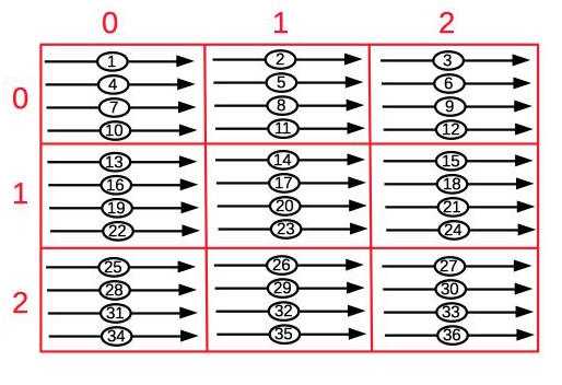
Therefore, we instead store 2-D data into a 1-D array of contiguous elements. The "row-major" scheme consists in storing rows in sequence. In other terms, if the width of the image is N, then pixel (i,j) is stored as Array[i * N + j]. This is actually the scheme used by the C language to store 2-D arrays.


Now that the program computes the Julia set pixels as a 1-D array of 3-byte elements, it would be nice to see them (if only to check that they're set correctly). So let's move on to Step #2...

Augment your program so that it saves the image to a file called julia.bmp, which stores the image in the bmp format. A bmp file consists of two parts:

A header
The 3-byte pixels of the image, in a row-major fashion

To make the above easier you are first provided with a helper C function, write_bmp_header(), which writes to a file the 40-byte header required for a bmp file. [Download source of write_bmp_header()]

See the source of write_bmp_header()...
/* write_bmp_header():
 *
 *   In:
 *      f: A file open for writing ('w') 
 *      (width, height): image dimensions
 *   
 *   Return:
 *      0 on success, -1 on failure
 *
 */

int write_bmp_header(FILE *f, int width, int height) {

  unsigned int row_size_in_bytes = width * 3 + 
	  ((width * 3) % 4 == 0 ? 0 : (4 - (width * 3) % 4));

  // Define all fields in the bmp header
  char id[3] = "BM";
  unsigned int filesize = 54 + (int)(row_size_in_bytes * height * sizeof(char));
  short reserved[2] = {0,0};
  unsigned int offset = 54;

  unsigned int size = 40;
  unsigned short planes = 1;
  unsigned short bits = 24;
  unsigned int compression = 0;
  unsigned int image_size = width * height * 3 * sizeof(char);
  int x_res = 0;
  int y_res = 0;
  unsigned int ncolors = 0;
  unsigned int importantcolors = 0;

  // Write the bytes to the file, keeping track of the
  // number of written "objects"
  size_t ret = 0;
  ret += fwrite(id, sizeof(char), 2, f);
  ret += fwrite(&filesize, sizeof(int), 1, f);
  ret += fwrite(reserved, sizeof(short), 2, f);
  ret += fwrite(&offset, sizeof(int), 1, f);
  ret += fwrite(&size, sizeof(int), 1, f);
  ret += fwrite(&width, sizeof(int), 1, f);
  ret += fwrite(&height, sizeof(int), 1, f);
  ret += fwrite(&planes, sizeof(short), 1, f);
  ret += fwrite(&bits, sizeof(short), 1, f);
  ret += fwrite(&compression, sizeof(int), 1, f);
  ret += fwrite(&image_size, sizeof(int), 1, f);
  ret += fwrite(&x_res, sizeof(int), 1, f);
  ret += fwrite(&y_res, sizeof(int), 1, f);
  ret += fwrite(&ncolors, sizeof(int), 1, f);
  ret += fwrite(&importantcolors, sizeof(int), 1, f);

  // Success means that we wrote 17 "objects" successfully
  return (ret != 17);
}

Second, here is a code fragment that shows how to write the pixels in a 1-D pixed array to a bpm file (opened as file output_file) after the header has been written:

// Writing the pixels after the header
for (y=0; y < height; y++) {
  for (x=0; x < width; x++) {
    fwrite(&(pixels[y * 3 * width + x * 3]), sizeof(char), 3, output_file);
  }
  // padding in case of an even number of pixels per row
  unsigned char padding[3] = {0,0,0};
  fwrite(padding, sizeof(char), ((width * 3) % 4), output_file);
}

Given the above, it should be straightforward to augment your program so that it produces a bmp file of the Julia set. Verify that the produced image is as shown below (by opening in whatever image viewing application, or a Web browser):

Once this is done, you are ready to go on to Activity #2, in which we make the program parallel!

In this activity we develop a parallel implementation of the program using a simple 1-D data distribution. We break it down into the three steps below:

The first step when designing a distributed-memory program is to pick a particular "data distribution", i.e., a way in which the data (input and or output) is split across the participating processes. In our Julia set program, the only data is the output image, and we opt for a simple and popular data-distribution scheme: a 1-D data-distribution. Simply put, we logically split our image into slabs and each process computes one slab.

Because in the previous activity we used a row-major storing scheme for our image, it makes sense to pick horizontal slabs. Our image has n rows of pixels (recall that n is the integer command-line argument). Let us first compute the data distribution, without computing the Julia set at all. The idea is that, based on its rank, each process must figure out which rows it will compute.

Implement a C (or C++) MPI program called 1D_parallel_julia (source file 1D_parallel_julia.c) that:

Takes a single command-line argument, n, an integer that's strictly positive.
Has each process print out its rank (out of how many processes in total), and which rows of the image (as a range) it should compute (but actually do nothing for now). See the sample executions below to see what kind of output is expected.
The intended data distribution should be in as many "slabs" as there are processes, where each process is in charge of a set of contiguous rows.

For simplicity, you can assume that the number of processes divides n, so that all processes have the same exact number of rows to compute. For more of a challenge, you may want to make sure that the distribution is as balanced as possible (at most a difference of one row between two processes). This can be done using discrete math so that everything is computed by a single formula, but can also be done programmatically with a loop (i.e., "counting by hand").

Run your program on this simple simulated 64-node cluster (download simple_cluster.xml and simple_cluster_hostfile.txt).


Below are a few sample executions of the program (this version of the program does not assume that the number of processes divides n, and enforces a "as balanced as possible" data distribution):

See a sample execution with 5 processes for n=1000 ...
As expected, each process process should process 200 rows:
% smpicc -O3 1D_parallel_julia.c -o 1D_parallel_julia
% smpirun -np 5 -hostfile ./simple_cluster_hostfile.txt -platform ./simple_cluster.xml ./1D_parallel_julia 1000
[Process 0 out of 5]: I should compute pixel rows 0 to 199, for a total of 200 rows
[Process 1 out of 5]: I should compute pixel rows 200 to 399, for a total of 200 rows
[Process 2 out of 5]: I should compute pixel rows 400 to 599, for a total of 200 rows
[Process 3 out of 5]: I should compute pixel rows 600 to 799, for a total of 200 rows
[Process 4 out of 5]: I should compute pixel rows 800 to 999, for a total of 200 rows
See a sample execution with 16 processes for n=100 ...
Note that the distribution is balanced, meaning that the number of rows differs by at most 1 across processors. This is not the only possible balanced data distribution (e.g., process 0 could compute only 6 rows, while process 15 could compute 7 rows).
% smpicc -O3 1D_parallel_julia.c -o 1D_parallel_julia
% smpirun -np 16 -hostfile ./simple_cluster_hostfile.txt -platform ./simple_cluster.xml ./1D_parallel_julia 100
[Process 0 out of 16]: I should compute pixel rows 0 to 6, for a total of 7 rows
[Process 1 out of 16]: I should compute pixel rows 7 to 13, for a total of 7 rows
[Process 2 out of 16]: I should compute pixel rows 14 to 20, for a total of 7 rows
[Process 3 out of 16]: I should compute pixel rows 21 to 27, for a total of 7 rows
[Process 4 out of 16]: I should compute pixel rows 28 to 33, for a total of 6 rows
[Process 5 out of 16]: I should compute pixel rows 34 to 39, for a total of 6 rows
[Process 6 out of 16]: I should compute pixel rows 40 to 45, for a total of 6 rows
[Process 7 out of 16]: I should compute pixel rows 46 to 51, for a total of 6 rows
[Process 8 out of 16]: I should compute pixel rows 52 to 57, for a total of 6 rows
[Process 9 out of 16]: I should compute pixel rows 58 to 63, for a total of 6 rows
[Process 10 out of 16]: I should compute pixel rows 64 to 69, for a total of 6 rows
[Process 11 out of 16]: I should compute pixel rows 70 to 75, for a total of 6 rows
[Process 12 out of 16]: I should compute pixel rows 76 to 81, for a total of 6 rows
[Process 13 out of 16]: I should compute pixel rows 82 to 87, for a total of 6 rows
[Process 14 out of 16]: I should compute pixel rows 88 to 93, for a total of 6 rows
[Process 15 out of 16]: I should compute pixel rows 94 to 99, for a total of 6 rows
See a sample execution with 16 processes for n=12 ...
Note that because n is small, some processes have nothing to do. (We don't care what these processes print as their range of rows).
% smpicc -O3 1D_parallel_julia.c -o 1D_parallel_julia
% smpirun -np 16 -hostfile ./simple_cluster_hostfile.txt -platform ./simple_cluster.xml ./1D_parallel_julia 100
[Process 1 out of 16]: I should compute pixel rows 1 to 1, for a total of 1 rows
[Process 2 out of 16]: I should compute pixel rows 2 to 2, for a total of 1 rows
[Process 3 out of 16]: I should compute pixel rows 3 to 3, for a total of 1 rows
[Process 4 out of 16]: I should compute pixel rows 4 to 4, for a total of 1 rows
[Process 5 out of 16]: I should compute pixel rows 5 to 5, for a total of 1 rows
[Process 6 out of 16]: I should compute pixel rows 6 to 6, for a total of 1 rows
[Process 7 out of 16]: I should compute pixel rows 7 to 7, for a total of 1 rows
[Process 8 out of 16]: I should compute pixel rows 8 to 8, for a total of 1 rows
[Process 9 out of 16]: I should compute pixel rows 9 to 9, for a total of 1 rows
[Process 10 out of 16]: I should compute pixel rows 10 to 10, for a total of 1 rows
[Process 11 out of 16]: I should compute pixel rows 11 to 11, for a total of 1 rows
[Process 12 out of 16]: I should compute pixel rows 12 to 11, for a total of 0 rows
[Process 13 out of 16]: I should compute pixel rows 12 to 11, for a total of 0 rows
[Process 14 out of 16]: I should compute pixel rows 12 to 11, for a total of 0 rows
[Process 15 out of 16]: I should compute pixel rows 12 to 11, for a total of 0 rows

Augment your program so that each process allocates space to store the pixels it needs to compute, and then computes them. A process must only allocate space for the pixels it needs to compute. In practice, each process runs on a different hosts, and one wishes to compute a large image that does not fit in the memory of a single host (which is one of the main motivations for going the "distributed-memory computing" route).

Have each process print its rank and time (using MPI_Wtime(), which returns a double) right before performing the computation and right after performing the computation!. Our cluster is not completely homogeneous, and these (simulated) times will show it.

The main difficulty here is keeping local vs. global indexing straight. That is, although as programmers we think of the image as an array of, say, N pixels, no N-pixel array is ever allocated in the program (only smaller arrays allocated by each process).

See more details about this local/global indexing thing ...

One of the difficulties of distributed-memory computing is just that... well... memory is distributed. Say my sequential non-distributed-memory program processes 2000 items. I can simply store them in a 2000-item array. Say now that I need to use distributed-memory computing (perhaps 2000 items don't fit in the memory of a single host, perhaps I just want to compute faster). I now use 20 hosts instead of 1, and on each host one process runs and allocates memory for 100 items. So, at each process I allocate a 100-item array. So far, so good.

The problem is that when my sequential program says "process item #i", for some i between 0 and 1999, I need to figure out two things:

Which process holds item #i?
In that process' item array, at which index is item #i stored?

The answer to the above depends on the data distribution! Say that process 0 (i.e., process with rank 0) holds items 0 to 99 (global indices), process 1 holds items 100 to 199 (global indices), etc. So, for a given i between 0 and 1999, with this data distribution, I have:

Item #i is held by process with rank i/100
At that process, item #i is store at index i%100 of the item array

i%100 ("i modulo 100") above is called the local index (i.e., where the element is stored in the array declared locally in the process), as opposed to i which is the global index.

The more complicated the distribution, the more intricate the global-to-local or local-to-global conversion. 1-D data distributions, like the one above, are the simplest. In the next activity we'll deal with a 2-D data distribution.

Augment your program so that the Julia set is saved to a bmp file. This requires some coordination between the processes:

Only one process must create the file and write the header
Processes need to write pixel rows in sequence, one after the other
It's probably a good idea to have the file opened in only a single process at a time

First you must pick one process to create the file and write the header to it (it is typical to pick process of rank 0). Second, each process, after its done computing its pixels, waits for a "go ahead!" message from its predecessor, writes to the file, and then sends a "go ahead!" message to its successor. The exceptions are the process with rank 0, which does not need to wait for a message, and the last process, which does not need to send a message. It doesn't really matter what these messages contain (e.g., they can be a single byte, or even zero-byte messages), as the whole purpose is to just have processes wait for their predecessors, not really receive meaningful data from them.

Warning: Make sure that your processes compute in parallel. That is, all processes compute together, and then they take turn writing what they have computed to the file.

Experiment with different numbers of processors and different values of n, and check that your bmp file is correct (valid, and contains the correct image).

What are logical topologies???

Although the above scheme is pretty simple, what we are really doing is creating a logical topology. That is, based on process rank, we impose structure on our set of processes. In this case, a "linear chain" in which process #i communicates with process #i+1. Probably the simplest structure. We will see examples of more complex logical topologies. Different applications lend themselves naturally to different logical topologies (rings, grids, trees, etc.). One interesting question, which is outside the score of this topic, is how well the logical topology matches the physical topology of the actual parallel platform in use (a good match typically boosts performance). Ideally, one can define a logical topology that makes writing the application easy, and that is also well-matched to the physical platform.

In this activity we develop a parallel implementation of the program using a "2-D data distribution". Just like for the previous activity, we break it down into the three steps below:

We now implement our parallel Julia set application using a 2-D data distribution. This means that each process now is in charge of a tile of the image in a logical checkerboard pattern. To make things simple we assume two things:

the total number of processes used is always a perfect square, p2
n, the image height, is perfectly divisible by p

These assumptions will not change the spirit of the program, but simplify its implementation significantly. This is because each process is responsible for a tile of the image with height n/p and width 2n/p. This is the amount of memory each process should allocate.

This 2-D data distribution complicates the global vs. local indexing issue that was discussed in Activity #2. The first thing to do is to figure out which process is responsible for which tile. A common approach is to use a row-major view of the processes. In other words, we think of a logical topology in which the processes are organized in a square grid (because our number of processes is a perfect square). By default, MPI gives us only a linear (i.e., 1-D) rank. We "transform" this rank into a 2-D rank where each process has a "row" and a "column", using a row-major scheme. This can be done with a little bit of discrete math (alternately, MPI provides a MPI_Cart_coords function that does this for you). Based on its 2-D coordinates, a process now knows which tile is is responsible for.

See an example...

Let's say our image has height 300 and width 600, and that we are using 9 processes. Each process then is responsible for a 100x200 tile. Let's see this on a "picture":

global index ranges cols [0-199] cols [200-399] cols [400-599]
rows [0-99] rank: 0
2-D rank: (0,0)
rank: 1
2-D rank: (0,1)
rank: 2
2-D rank: (0,2)
rows [100-199] rank: 3
2-D rank: (1,0)
rank: 4
2-D rank: (1,1)
rank: 5
2-D rank: (1,2)
rows [200-299] Rank: 6
2-D rank: (2,0)
Rank: 7
2-D rank: (2,1)
Rank: 8
2-D rank: (2,2)

Every white cell above represents a tile. The (global) row and column index ranges for the pixels in the tile are shown in the first row/column. In each tile is shown the rank of the process that owns it, and the 2-D rank of this process (computed based in the process rank and p). For instance, process of rank 5 has 2-D rank (1,2), meaning that it is in the 2nd row and the 3rd column of the logical 3x3 process grid. As such, it is responsible for image pixels between rows 100 and 199 and between columns 400 and 599. In "array slice notation, this would be [100:199, 400:599].

Implement a program called 2D_parallel_julia (source 2D_parallel_julia.c) that does not allocate memory or compute anything for now, but that merely has each process print out its rank, it's 2-D rank, and the pixel row and column ranges for which it is responsible.

Run your program on this simple simulated 64-node cluster (download simple_cluster.xml and simple_cluster_hostfile.txt). These are the same files are for Activity #1.


Below are a few sample executions of the program:

See a sample execution with 9 processes for n=30 ...
% smpicc -O3 2D_parallel_julia.c -o 2D_parallel_julia
% smpirun -np 9 -hostfile ./simple_cluster_hostfile.txt -platform ./simple_cluster.xml ./1D_parallel_julia 30
[Process rank 0]: my 2-D rank is (0, 0), my tile is [0:9, 0:19]
[Process rank 1]: my 2-D rank is (0, 1), my tile is [0:9, 20:39]
[Process rank 2]: my 2-D rank is (0, 2), my tile is [0:9, 40:59]
[Process rank 3]: my 2-D rank is (1, 0), my tile is [10:19, 0:19]
[Process rank 4]: my 2-D rank is (1, 1), my tile is [10:19, 20:39]
[Process rank 5]: my 2-D rank is (1, 2), my tile is [10:19, 40:59]
[Process rank 6]: my 2-D rank is (2, 0), my tile is [20:29, 0:19]
[Process rank 7]: my 2-D rank is (2, 1), my tile is [20:29, 20:39]
[Process rank 8]: my 2-D rank is (2, 2), my tile is [20:29, 40:59]
See a sample execution with 16 processes for n=200 ...
% smpicc -O3 2D_parallel_julia.c -o 2D_parallel_julia
% smpirun -np 16 -hostfile ./simple_cluster_hostfile.txt -platform ./simple_cluster.xml ./2D_parallel_julia 200
[Process rank 0]: my 2-D rank is (0, 0), my tile is [0:49, 0:99]
[Process rank 1]: my 2-D rank is (0, 1), my tile is [0:49, 100:199]
[Process rank 2]: my 2-D rank is (0, 2), my tile is [0:49, 200:299]
[Process rank 3]: my 2-D rank is (0, 3), my tile is [0:49, 300:399]
[Process rank 4]: my 2-D rank is (1, 0), my tile is [50:99, 0:99]
[Process rank 5]: my 2-D rank is (1, 1), my tile is [50:99, 100:199]
[Process rank 6]: my 2-D rank is (1, 2), my tile is [50:99, 200:299]
[Process rank 7]: my 2-D rank is (1, 3), my tile is [50:99, 300:399]
[Process rank 8]: my 2-D rank is (2, 0), my tile is [100:149, 0:99]
[Process rank 9]: my 2-D rank is (2, 1), my tile is [100:149, 100:199]
[Process rank 10]: my 2-D rank is (2, 2), my tile is [100:149, 200:299]
[Process rank 11]: my 2-D rank is (2, 3), my tile is [100:149, 300:399]
[Process rank 12]: my 2-D rank is (3, 0), my tile is [150:199, 0:99]
[Process rank 13]: my 2-D rank is (3, 1), my tile is [150:199, 100:199]
[Process rank 14]: my 2-D rank is (3, 2), my tile is [150:199, 200:299]
[Process rank 15]: my 2-D rank is (3, 3), my tile is [150:199, 300:399]

Augment your program so that each process allocates space to store the pixels it needs to compute, and then computes them. As in the previous activity, the main difficulty here is keeping local vs. global indexing straight. It is a bit more complex than for Activity #2 due to the use of a 2-D data distribution.

Have each process apply a tint to the pixels it handles, by passing value rank2 (i.e., the square of the rank) as the 5th argument to function compute_julia_pixel() (instead of passing the default 1.0 value).

Augment your program so that the Julia set is saved to a bmp file. The difference with Activity #2 is that now each process holds a tile, and yet the file must contain the pixels in row major order. So each process will have to append many times to the file, writing one piece of a row at a time. As a result, more complex coordination is required compared to Activity #2.

See a visual example/explanation ...

The figure above shows an example with 9 processes (2-D rank coordinates are shown in red), where each process holds a 4x8 tile (4 row segments). The numbers on each segment indicate the sequence in which the pixels must be written to the file. In this example, there are 36 row segments. First process (0,0) writes its first segment, then process (0,1) writes its first segment, etc. For instance, at step 20, process (1,1) writes its third segment. You must implement the "go ahead!" messaging scheme so that the processes write to the file in the correct order.
Using a tint of 1.0 at each process, this program should produce the same images as that in Activity #2 (which can be useful for debugging). When using rank2, one sees a checkered pattern. Here is a sample image generated with 9 processors for n=300:

What have we learned?

Congratulations for making it this far. At this point you have learned how to design a distributed-memory application as an SMPD program using SMPI, have been exposed to both 1-D and 2-D data distributions, and have learned how to use communication to orchestrate the executions of MPI processes. You may also have learned about memory layouts of 2-D arrays.

Our Julia set computation is a "toy application". Admittedly, our use of a 2-D data distribution made the application more complicated to write without any clear benefit. We will see other examples for which 2-D data distributions provide significant performance advantages. Also, we handled all file I/O "by hand". In practice, MPI provides a set of abstractions and functions to perform parallel I/O, called MPI IO, that could be used to achieve better performance on a real systems with high-performance parallel file systems.

What was difficult?

In a README file write a brief "essay" explaining what you found surprising/challenging, and what solutions you used to solve your difficulties. Are you happy with your implementations? Do you see room for improvement?

The End