Objective: To implement the "outer product" matrix multiplication algorithm in a distributed memory manner using message passing.
For this module, we use a 2-D block data distribution.
More precisely, we consider the C = A×B multiplication
where all three matrices are square of dimensions N×N. All matrices
contain double precision elements (double).
The execution takes place on p processors, where p is a perfect square and √p
divides N. Each processor thus holds a
N/√p × N/√p square block of each matrix.
For instance, with N=6, consider the example matrix A as shown below:
        10 20 30 40 50 60
        11 21 31 41 51 61
        12 22 32 42 52 62
        13 23 33 43 53 63
        14 24 34 44 54 64
        15 25 35 45 55 65
Now let's assume that p=4. The 4 processes are logically organized in a 2x2 grid (hence the name of the data distribution) in row-major order as follows:
| process #0 | process #1 |
| process #2 | process #3 |
In this setup, for instance, process #0 holds the following 3x3 block of matrix A:
        10 20 30
        11 21 31
        12 22 32
and process #3 holds the following 3x3 block of matrix A:
        43 53 63
        44 54 64
        45 55 65
At process #3, element with value 54 has local indices (1,1), but its global indices are (4,4), assuming that indices start at 0.
This module consists of 2 activities, each described in its own tab above, which should be done in sequence:
You should turn in a single archive (or a github repo) with:
Implement an MPI program called matmul_init (matmul_init.c) that takes a
single command-line argument, N, which is a strictly positive integer. N is the
dimension of the square matrices that we multiply. Your program should check that the number of processes
is a perfect square, and that its square root divides N (printing an error message and exiting if this is
not the case).
The objective of the program is for each process to allocate and initialize its block of each matrix. We multiply particular matrices, defined by:
Ai,j = i and Bi,j = i + j.
The above is with global indices, which go from 0 to N-1.
Given the above definitions of A and B, there is a simple analytical solution for C. There is thus a closed-form expression for the sum of the elements of C: N3 (N - 1)2 / 2. You will use this formula to check the validity of your matrix multiplication implementation in Activity #2.
Have each process allocate its blocks of A, B, and C, initialize its blocks of A and B to the appropriate values, and then print out the content of these blocks. Each process should print its MPI rank (the "linear rank") as well as its 2-D rank, which is easy to determine based on the linear rank.
For instance, here is an excerpt from the output (that generated by the process of rank 2) for p=4 and N=8, using cluster_crossbar_64.xml as a platform file and hostfile_64.txt as a hostfile (since this module is about correctness, you can use pretty much any such valid files).
% smpirun -np 4 \
          -platform cluster_crossbar_64.xml \
          -hostfile hostfile_64.txt \
          ./matmul_init 8
[...]
Process rank 2 (coordinates: 1,0), block of A:
4.0 4.0 4.0 4.0
5.0 5.0 5.0 5.0
6.0 6.0 6.0 6.0
7.0 7.0 7.0 7.0
Process rank 2 (coordinates: 1,0), block of B:
4.0 5.0 6.0 7.0
5.0 6.0 7.0 8.0
6.0 7.0 8.0 9.0
7.0 8.0 9.0 10.0
[...]
Note that due to the convenience of simulation, the output from one process will never be interleaved with the output of another process. If you run this code "for real" with MPI, instead of SMPI, output will be interleaved and additional synchronization will be needed to make the output look nice. The order in which the processes output their blocks is inconsequential. You may want to use a barrier synchronization to first see all blocks of A and then all blocks of B though.
Obviously, we won’t run this program for large N. The goal is simply to make sure that matrix blocks are initialized correctly on all processes.
Implement a program called matmul (matmul.c), which builds on your matmul_init
program from the previous activity and implements the outer-product matrix multiplication algorithm.
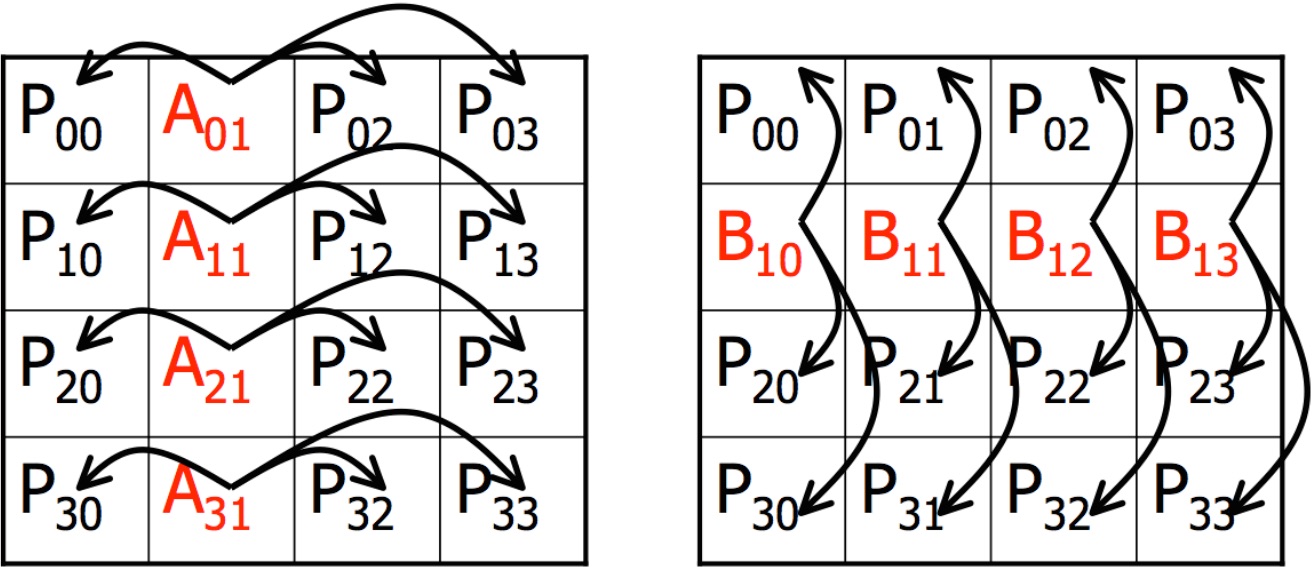
The principle of the outer-product algorithm, as might be expected, is that a matrix multiplication can be performed as a sequence of outer-products. You may have covered this algorithm in a course, and it is of course well-document in various texts. You may expand below to get a brief description of the algorithm, which should be sufficient for you do do this step even if you've never seen the outer-product algorithm before.
Implementing "broadcasts": The algorithm involves broadcasts in process rows and process columns. In MPI, a broadcast
must involve all processes in a communicator. Thus, one option to implement the
algorithm is to create 2p communicators, one for each process row and one for each
process column. MPI_Bcast can then be used for these communicators. Communicators
can be easily created using the MPI_Comm_split function (see the MPI documentation). The alternative
is to rely on sequences of point-to-point communications, which isn't as pretty and likely not as efficient.
Result validation: Recall that we compute a particular matrix product. To validate the result once the outer-product algorithm
has finished, each process must compute the sum of all the elements in its block of C. These sums are then
all added up together (using MPI_Reduce is the way to go), and the process of rank 0 prints out
the sum. This process then computes the difference with the analytical formula:
N3 (N - 1)2 / 2. This process should print out an error message if the
two values don't match (beware of casts and round-off; you likely want to do everything in double precision
and check that the absolute value of the difference of the two values is below some small epsilon, instead
of testing for equality with the '==' operator).
For debugging purposes, remember that it's a good idea to insert calls to MPI_Barrier
so that debugging output from the program can be structured step-by-step.
Congratulations for making it this far. You have learned to implement a moderately complex algorithm using 2-D data distribution and communication patterns that involve subset of the processes. This algorithm and its implementation are very typical of parallel numerical linear algebra implementations, and is among the simplest. Topic #4 contains a module in which we use your implementation as a starting point and explore performance issues, with the goal of reducing the performance penalty of communications.
In a README file write a brief "essay" explaining what you found surprising/challenging, and what solutions you used to solve your difficulties. Are you happy with your implementations? Do you see room for improvement?